Stefano Costa

There's more than potsherds out here

Faccio l’archeologo e vivo a Genova

Categoria: IOSACal

  • Install iosacal with conda

    Starting today, you can install iosacal with conda. This adds to the existing installation procedure with pip. Conda is a good fit for complex projects and has better tooling for reproducibility.

    Installing iosacal can be achieved by adding conda-forge to your channels with:

    conda config --add channels conda-forge conda config --set channel_priority strict

    Once the conda-forge channel has been enabled, iosacal can be installed with conda:

    conda install iosacal

    or with mamba:

    mamba install iosacal
  • IOSACal in Google Colab

    Google Colab is a popular notebook service that you can run directly from your browser. Python is natively supported and it’s fairly easy to run a Jupyter notebook, even with custom dependencies like Numpy and Matplotlib.

    You can run IOSACal in Google Colab! I have added a new short how-to guide in the official documentation. Find the how-to at https://iosacal.readthedocs.io/en/latest/google_colab.html.

    This takes advantage of a demo notebook that was contributed by Jelmer Wind.

    A screenshot of the demo notebook running IOSACal in Google Colab. Even with a plot!

  • Research papers and case studies using iosacal

    Research papers and case studies using iosacal

    I have updated the documentation of iosacal with a new page that lists all research papers and case studies where the software gets a mention for being used.

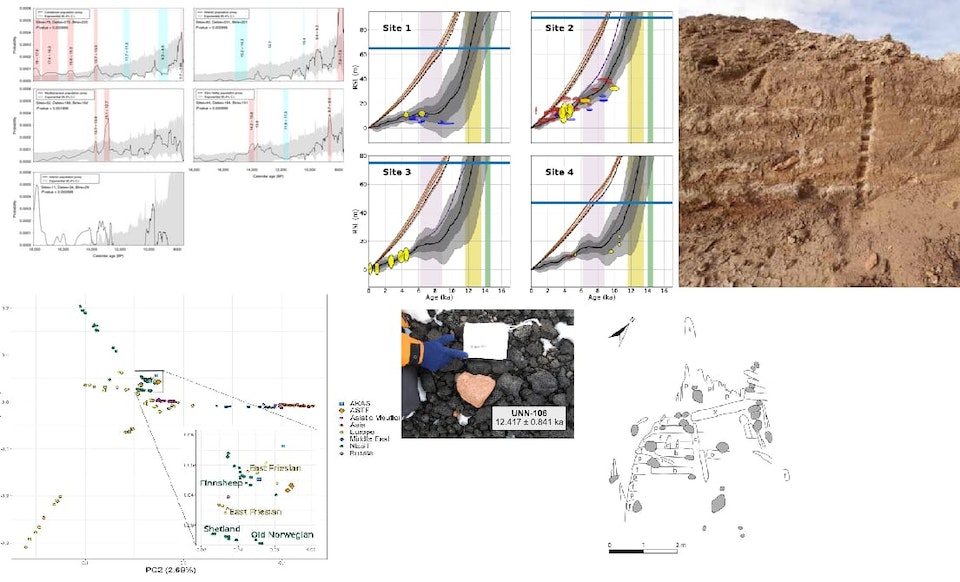
    A collage of figures from the papers using iosacal

    The list is at https://iosacal.readthedocs.io/en/latest/literature.html and it’s longer than I thought, with 6 papers ranging from Norway to Antarctica, from the Last Glacial Maximum to the European Middle Ages.

    It’s humbling to see this small piece of software find its way in so many research projects and I’m learning a lot by studying these publications.

    Some authors contributed to iosacal with new features and bug fixes, and that is the most accurate metric of a healthy project that I can think of.

    I’m going to add more useful content to the documentation as the main focus of the 0.7 release. In the meantime, you can continue using iosacal 0.6 in your research projects.

  • IOSACal 0.6 released with new features for simulation and quantiles

    I’m happy to announce that IOSACal version 0.6 was released on October 1st, 2022.

    IOSACal 0.6 brings new features for simulating radiocarbon dates and obtaining quantiles, added respectively by Hythem Sidky and Roger Creel, who both contributed to IOSACal for the first time. I want to thank both for their efforts to share improvements to the IOSACal source code by sticking to the code of conduct and contribution rules of the project.

    The documentation at https://iosacal.readthedocs.io/ has been updated substantially, and some pages are now generated directly from Jupyter notebooks. You can download those notebooks and quickly start working on your own research notebooks.

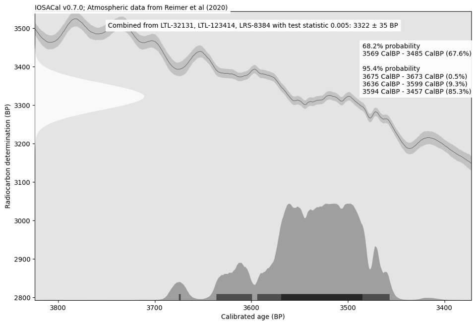
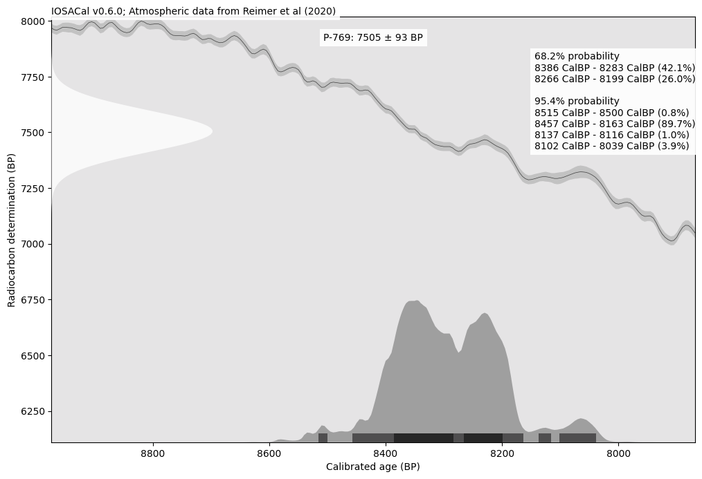
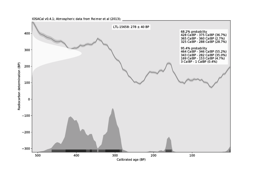
    Calibrated radiocarbon date plot created with IOSACal

    You can get this update as usual with pip install iosacal or by updating your requirements.txt to this version:

    iosacal==0.6.0

    IOSACal 0.6 brings several improvements to the development process, most notably continuous integration (CI) thanks to Codeberg CI. All pull requests are automatically run through iosacal’s own test suite (coverage is not yet complete but it is improving). The detailed list of all changes is at https://iosacal.readthedocs.io/en/stable/whatsnew.html

    The demo web application was discontinued, and usage with MyBinder or Google Colab is now encouraged.

    That’s it for now, development continues at https://codeberg.org/steko/iosacal!

    This article is also available via the new IOSACal updates newsletter!

  • IOSACal 0.5, featuring IntCal20 and more

    After three years of slow paced development, IOSACal 0.5 is here. The DOI of the latest release is https://doi.org/10.5281/zenodo.630455

    As before, the preferred installation method is with pip in a virtual environment. The documentation is at https://iosacal.readthedocs.io/

    This release brings the new IntCal20 calibration data and several improvements for different use cases, plus one important bug fix. Apart from myself, there were two contributors to this release, I’m grateful to Karl Håkansson and Wesley Weatherbee for their work.

    These are the highlights from the release notes:

    • the project has moved to Codeberg for source code hosting and issue tracking. The new Git repository is at https://codeberg.org/steko/iosacal with a default branch name of main
    • there is an official Code of Conduct that all contributors (including the maintainter) will need to follow, based on Contributor Covenant
    • the documentation has seen some improvements, in particular in the Contributing section. Overall, making contributions easier from both expert and novice users is a major theme in this release.
    • interactive use in Jupyter notebooks is made easier with CalibrationCurve that can be created in many ways (such as loading from an arbitrary file, or from a standard calibration curve called by shorthand)
    • fixed a bug that made plots with AD/CE setting incorrect (contributed by Karl Håkansson)
    • fixed a bug that caused a wrong plot density function for dates 80 BP to 0 BP (contributed by Karl Håkansson)
    • add IntCal20 calibration data (contributed by Wesley Weatherbee)

    On the technical side:

    • the command line interface is now based on the Click library
    • most code is now covered by tests, based on pytest
    • Python 3.6 or above required
    • requires Numpy 1.18 and Matplotlib 3.0

    I don’t have big plans for the next release. I would like to add more tests, modernize the code and make it easier to adapt / tinker with. The only major achievement I’m looking forward to is to submit an article about IOSACal to the Journal of Open Source Software.

  • IOSACal on the web: quick calibration of radiocarbon dates

    IOSACal on the web: quick calibration of radiocarbon dates

    Update November 2022: the web app is now discontinued and the recommended way to run IOSACal in the browser is with Jupyter in MyBinder or Google Colab. See this issue for more details.

    The IOSA Radiocarbon Calibration Library (IOSACal) is an open source calibration software. IOSACal is meant to be used from the command line and installation, while straightforward for GNU/Linux users, is certainly not as easy as common desktop apps. To overcome this inconvenience, I dedicated some efforts to develop a version that is immediately usable.

    The IOSACal web app is online at https://iosacal.herokuapp.com/.

    This is a demo service, so it runs on the free tier of the commercial Heroku platform and it may take some time to load the first time you visit the website. It is updated to run with the latest version of the software (at this time, IOSACal 0.4.1, released in May).

    Since it may be interesting to try the app even if you don’t have a radiocarbon date at hand, at the click of a button you can randomly pick one from the open data Mediterranean Radiocarbon dates database, and the form will be filled for you.

    The random date picker in action
    The random date picker in action

    Unfortunately, at this time it is not possible to calibrate or plot multiple dates in the web interface (but the command-line program is perfectly capable of that).

    IOSACal Web is made with Flask and the Bootstrap framework, and the app itself is of course open source.

    IOSACal is written in the Python programming language and is based on Numpy, Scipy and Matplotlib. This work wouldn’t be possible without the availability of such high quality programming libraries.

  • IOSACal 0.4

    IOSACal 0.4

    IOSACal is an open source program for calibration of radiocarbon dates.

    A few days ago I released version 0.4, that can be installed from PyPI or from source. The documentation and website is at http://c14.iosa.it/ as usual. You will need to have Python 3 already installed.

    The main highlight of this release are the new classes for summed probability distributions (SPD) and paleodemography, contributed by Mario Gutiérrez-Roig as part of his work for the PALEODEM project at IPHES.

    A bug affecting calibrated date ranges extending to the present was corrected.

    On the technical side the most notable changes are the following:

    • requires NumPy 1.14, SciPy 1.1 and Matplotlib 2.2
    • removed dependencies on obsolete functions
    • improved the command line interface

    You can cite IOSACal in your work with the DOI https://doi.org/10.5281/zenodo.630455. This helps the author and contributors to get some recognition for creating and maintaining this software free for everyone.